In computer science, the method of contraction hierarchies is a speed-up technique for finding the shortest-path [Shortest path problem] in a graph [Graph]. The most intuitive applications are car-navigation systems: a user wants to drive from \(A\) to \(B\) using the quickest possible route. The metric optimized here is the travel time. Intersections are represented by vertices [Vertex], the road sections connecting them by edges. The edge weights represent the time it takes to drive along this segment of the road. A path from \(A\) to \(B\) is a sequence of edges (road sections); the shortest path is the one with the minimal sum of edge weights among all possible paths. The shortest path in a graph can be computed using Dijkstra’s algorithm but, given that road networks consist of tens of millions of vertices, this is impractical. Contraction hierarchies is a speed-up method optimized to exploit properties of graphs representing road networks. The speed-up is achieved by creating shortcuts in a preprocessing phase which are then used during a shortest-path query to skip over “unimportant” vertices. This is based on the observation that road networks are highly hierarchical. Some intersections, for example highway junctions, are “more important” and higher up in the hierarchy than for example a junction leading into a dead end. Shortcuts can be used to save the precomputed distance between two important junctions such that the algorithm doesn’t have to consider the full path between these junctions at query time. Contraction hierarchies do not know about which roads humans consider “important” (e.g. highways), but they are provided with the graph as input and are able to assign importance to vertices using heuristics.
[…]
The contraction hierarchies (CH) algorithm is a two-phase approach to the shortest path problem consisting of a preprocessing phase and a query phase. […]
Consider two large cities connected by a highway. Between these two cities, there is a multitude of junctions leading to small villages and suburbs. Most drivers want to get from one city to the other – maybe as part of a larger route – and not take one of the exits on the way. In the graph representing this road layout, each intersection is represented by a node and edges are created between neighboring intersections. To calculate the distance between these two cities, the algorithm has to traverse all the edges along the way, adding up their length. Precomputing this distance once and storing it in an additional edge created between the two large cities will save calculations each time this highway has to be evaluated in a query. This additional edge is called a “shortcut” and has no counterpart in the real world. The contraction hierarchies algorithm has no knowledge about road types but is able to determine which shortcuts have to be created using the graph alone as input.
Algorithm
Preprocessing phase

Node contraction
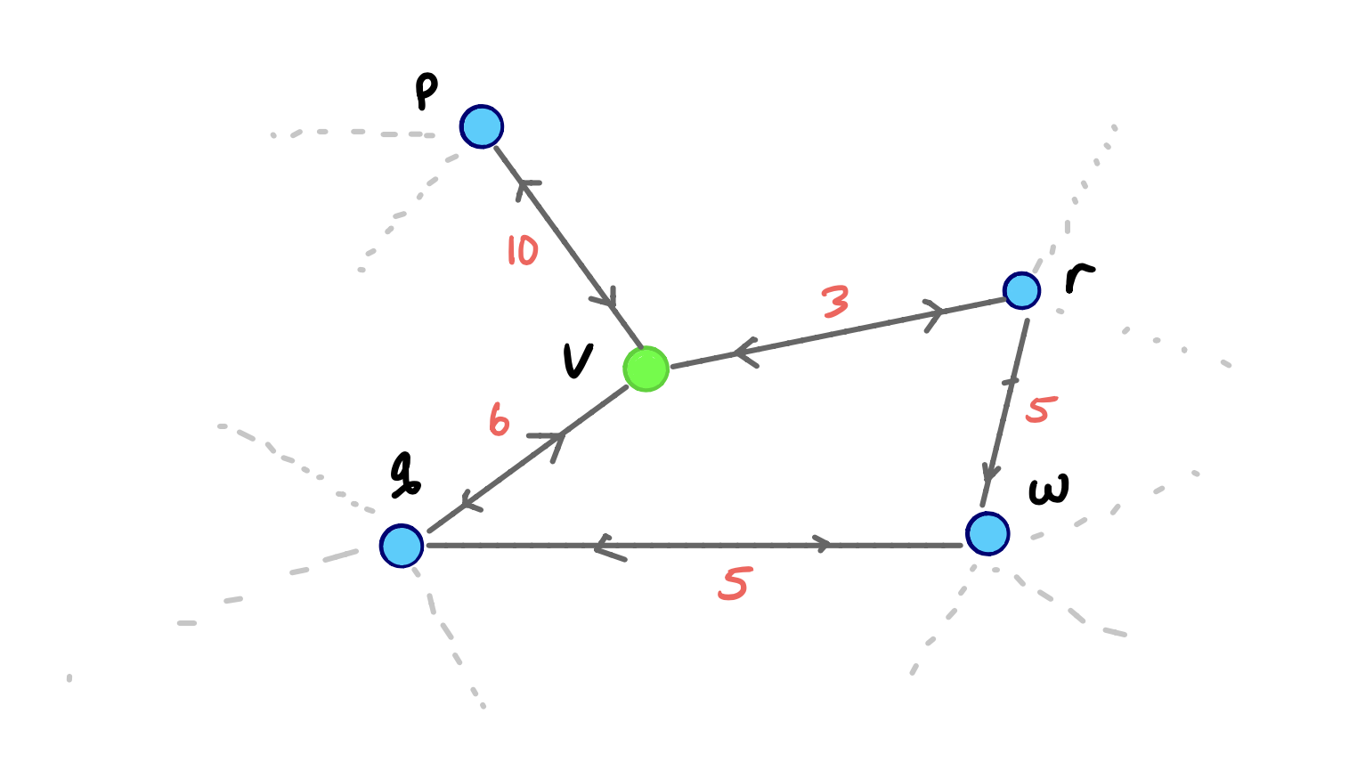
[Contraction hierarchies’] basic ingredient is the contraction of a node \(v\): The node \(v\) is removed from the graph, but for any pair of arcs \((u,v)\), \((v,w)\) such that \((u,v,w)\) is a shortest path, a shortcut arc \((u,w)\) with the cost of \((u,v,w)\) is inserted. The contracted node \(v\) is called the midpoint of the shortcut. The remaining graph has one less node, a changed set of arcs (some dropped, some added), and the same shortest paths between any two remaining nodes.
When contracting a vertex \(v\) it is temporarily removed from the graph \(G\), and a shortcut is created between each pair \(\{\u,w\}\) of neighboring vertices if the shortest path from \(u\) to \(w\) contains \(v\).
[…]
Consider a node \(v\) and the following
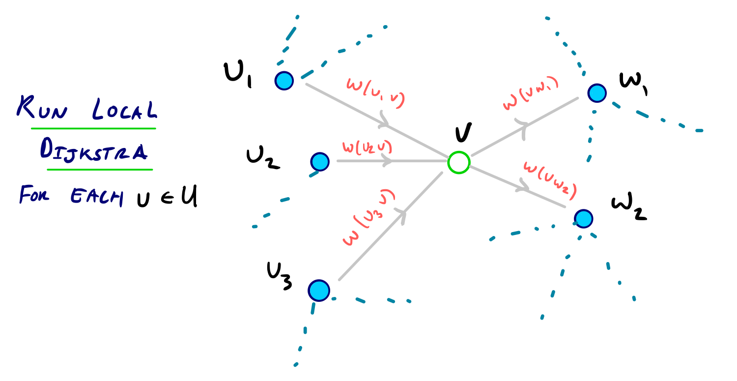
contractprocess:We denote the set of all vertices with edges incoming to \(v\) as \(U\), and the set of all vertices with incoming edges from \(v\) as \(W\).
Then for each pair of vertices \((u, w)\), for \(u\) in \(U\) and \(w\) in \(W\):
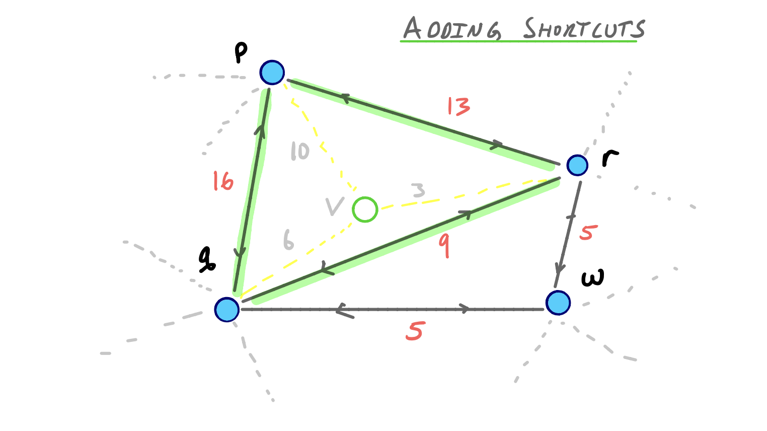
If the path <\(u,v,w\)> is the unique shortest path from \(u\) to \(w\), we add a shortcut edge \(u,w\) to the graph with weight \(w(u, v) + w(v, w)\).
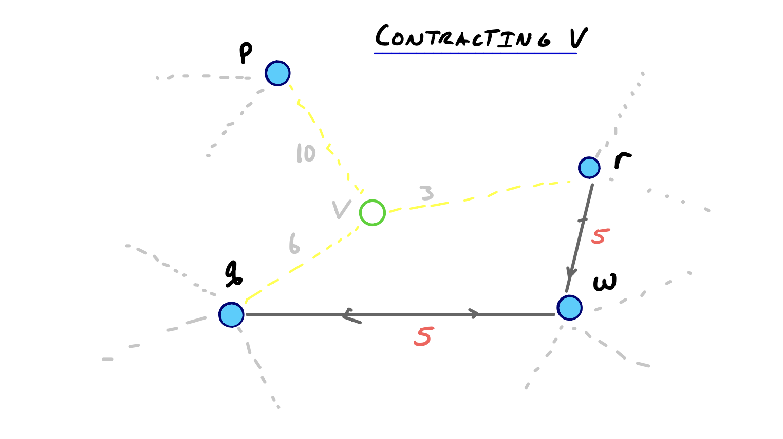
Then, we remove \(v\) and all of its adjacent edges from the graph.
We’re now done contracting \(v\).
When to add shortcuts
But in general, we need a method for efficiently determining when to add a shortcut edge.
[…]
So we can do the following:
- \(\forall\; u \in U\):
- \(\forall\; w \in W\):
- Compute \(P_{w} = \operatorname{weight}(u, v) + \operatorname{weight}(v, w)\)
- \(P_{max} = \operatorname{max}(P_w)\)
- \(\forall\; w \in W\):
- Perform a standard Dijkstra’s shortest-path [Single-pair shortest path problem] search from \(u\) [to \(w\)] on the subgraph excluding \(v\). Halt when we settle (1) a vertex with a shortest-path score \(> P_{max}\) or (2) \(w\).
- Add a shortcut if \(P_w < \operatorname{distance}(u, w)\)
- \(\forall\; w \in W\):
[paraphrased, formatting mine]
How to decide if a shortcut is strictly necessary?
- Naive: add all possible shortcuts.
- Strict: invoke Dijkstra and perform a “witness search” proof.
- Pragmatic: invoke Dijkstra with cutoffs (max cost, max hops).
- \(\forall\; u \in U\):
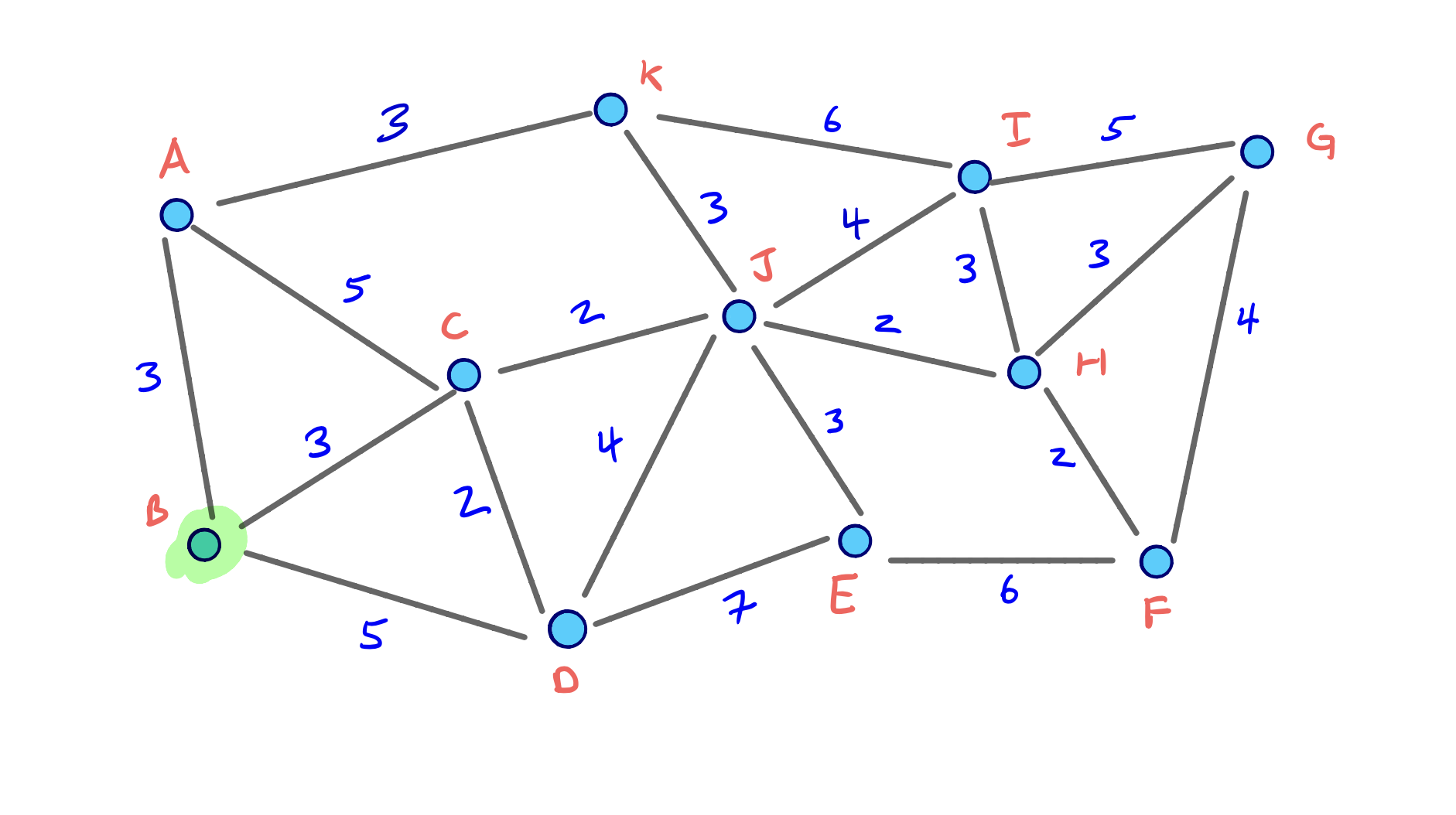
Example 1
Let:
- \(v\) be \(B\)
- \(U\) be \((A, C, D)\)
- \(W\) be \((A, C, D)\)
Steps to contract \(v (B)\):
- For each \(u \in U\):
- With \(u = A\):
- For each \(w \in W\):
- Skip \(w = A\)
- With \(w = C\):
\(P_{w} = \operatorname{weight}(u, v) + \operatorname{weight}(v, w)\)
\(P_{C} = weight(A, B) + weight(B, C) = 3 + 3 = 6\)
- With \(w = D\):
\(P_{w} = \operatorname{weight}(u, v) + \operatorname{weight}(v, w)\)
\(P_{D} = weight(A, B) + weight(B, D) = 3 + 5 = 8\)
- \(P_{max} = \operatorname{max}(P_{C}, P_{D}) = \operatorname{max}(6, 8) = 8\)
- For each \(w \in W\):
- Skip \(w = A\)
- With \(w = C\):
- Perform a standard Dijkstra’s shortest-path search from \(u (A)\) to \(w ( C)\) on the subgraph excluding \(v (B)\). Halt when we settle (1) a vertex with a shortest-path score \(> P_{max}\) or (2) \(w ( C)\).
- Settle \(K\) at a cost of \(3\) (\((A, K)\))
- Settle \(B\) at a cost of \(3\) (\((A, B)\))
- Settle \(C\) at a cost of \(5\) (\((A, C)\))
- Done!
- Don’t add a shortcut. \(P_{C} > \operatorname{distance}(A, C)\) (\(6 > 5\))
- Perform a standard Dijkstra’s shortest-path search from \(u (A)\) to \(w ( C)\) on the subgraph excluding \(v (B)\). Halt when we settle (1) a vertex with a shortest-path score \(> P_{max}\) or (2) \(w ( C)\).
- With \(w = D\):
- Perform a standard Dijkstra’s shortest-path search from \(u (A)\) to \(w (D)\) on the subgraph excluding \(v (B)\). Halt when we settle (1) a vertex with a shortest-path score \(> P_{max}\) or (2) \(w (D)\).
- Settle \(K\) at a cost of \(3\) (\((A, K)\))
- Settle \(B\) at a cost of \(3\) (\((A, B)\))
- Settle \(C\) at a cost of \(5\) (\((A, C)\))
- Settle \(J\) at a cost of \(6\) (\((A, K) + (K, J)\))
- Settle \(D\) at a cost of \(7\) (\((A, C) + (C, D)\))
- Don’t add a shortcut. \(P_{D} > \operatorname{distance}(A, D)\) (\(8 > 7\))
- Perform a standard Dijkstra’s shortest-path search from \(u (A)\) to \(w (D)\) on the subgraph excluding \(v (B)\). Halt when we settle (1) a vertex with a shortest-path score \(> P_{max}\) or (2) \(w (D)\).
- For each \(w \in W\):
- With \(u = C\):
- Left as an exercise. No shortcuts added.
- With \(u = D\):
- Left as an exercise. No shortcuts added.
- With \(u = A\):
Example 2
Let:
- \(v\) be \(K\)
- \(U\) be \((A, J)\)
- \(W\) be \((A, J)\)
Steps to contract \(v (K)\):
- For each \(u \in U\):
- With \(u = A\):
- For each \(w \in W\):
- Skip \(w = A\)
- With \(w = J\):
\(P_{w} = \operatorname{weight}(u, v) + \operatorname{weight}(v, w)\)
\(P_{J} = weight(A, K) + weight(K, J) = 3 + 3 = 6\)
- \(P_{max} = \operatorname{max}(P_{J}) = \operatorname{max}(6) = 6\)
- For each \(w \in W\):
- Skip \(w = A\)
- With \(w = J\):
- Perform a standard Dijkstra’s shortest-path search from \(u (A)\) to \(w (J)\) on the subgraph excluding \(v (K)\). Halt when we settle (1) a vertex with a shortest-path score \(> P_{max}\) or (2) \(w (J)\).
- Settle \(K\) at a cost of \(3\) (\((A, K)\))
- Settle \(C\) at a cost of \(5\) (\((A, C)\))
- Settle \(J\) at a cost of \(7\) (\((A, K) + (K, J)\))
- Done!
- Add a shortcut! \(P_{C} < \operatorname{distance}(A, J)\) (\(6 < 7\))
- Perform a standard Dijkstra’s shortest-path search from \(u (A)\) to \(w (J)\) on the subgraph excluding \(v (K)\). Halt when we settle (1) a vertex with a shortest-path score \(> P_{max}\) or (2) \(w (J)\).
- For each \(w \in W\):
- With \(u = J\):
- Left as an exercise. Adds a shortcut to make the shortcut connecting \((A, J)\) bidirectional.
- With \(u = A\):
Query phase
In the query phase, a bidirectional search is performed starting from the starting node \(s\) and the target node \(t\) on the original graph augmented by the shortcuts created in the preprocessing phase.
How to search the contraction hierarchy?
- Bi-directional search (two directions simultaneously)
- Bi-directional search (one direction at a time)
- Hybrid search (bi-directional first, then something else)
- Contraction hierarchies can also be combined with your favourite uni-directional search scheme (Harabor and Stuckey 2021)
[paraphrased]
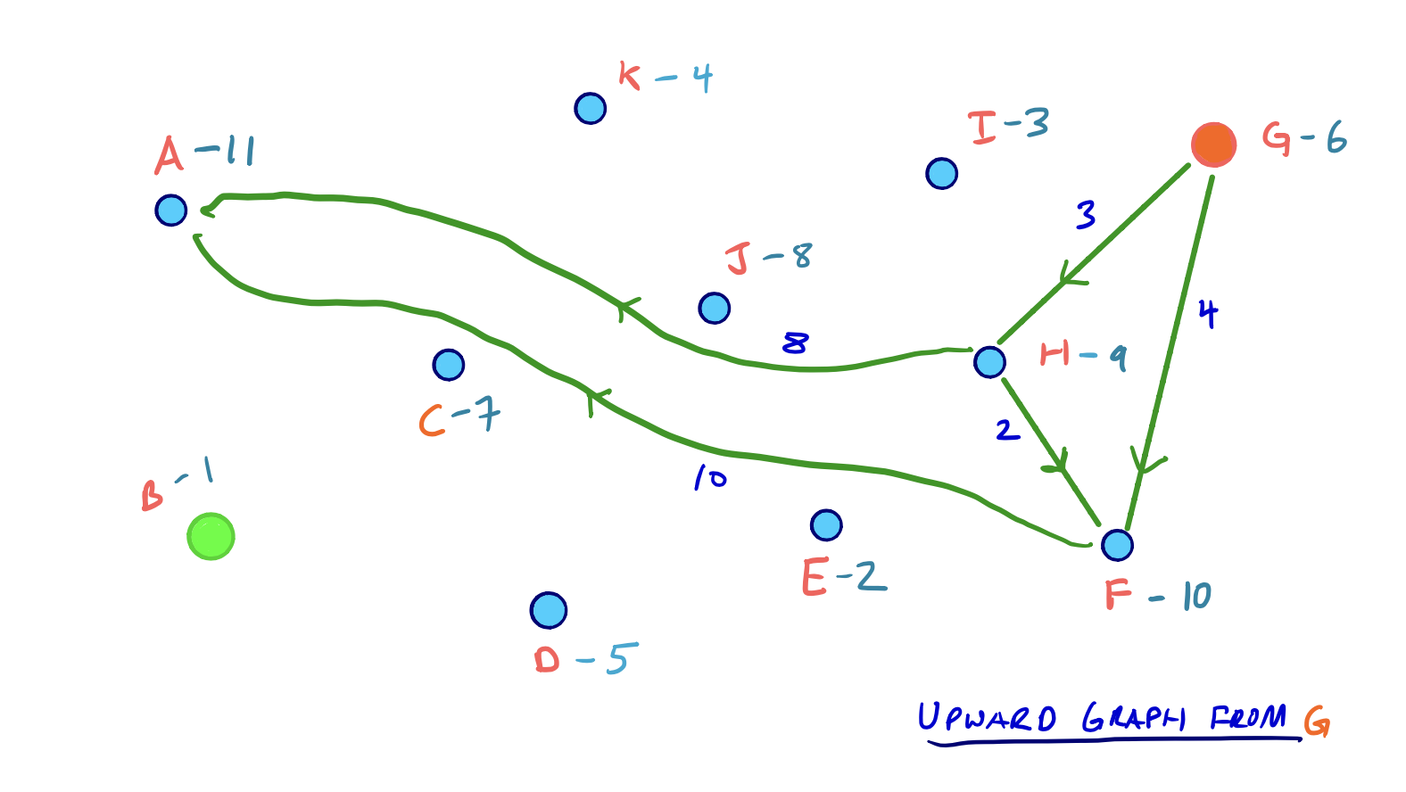
FIX; up/down is backward here. Check against (Geisberger et al. 2008)
- The upward graph only contains edges from \(v\) to \(w\) where we contracted \(v\) after \(w\).
- The downward graph only contains edges from \(v\) to \(w\) where we contracted \(v\) before \(w\).
[…]
For our [contraction hierarchies] query from \(s\) to \(t\), we run a forward search from \(s\) on [the upward] graph, and a backward search from \(t\) on the [downward] graph.
[paraphrased]
Example
[…]
[…] for symmetric graphs like the ones we are considering, a backward search (reversing edge directions) on \(G_{down}\) is the same as an upward search on \(G_{up}\). So from both our source and target nodes, we can perform a standard Dijkstra search on the \(G_{up}\) graph.
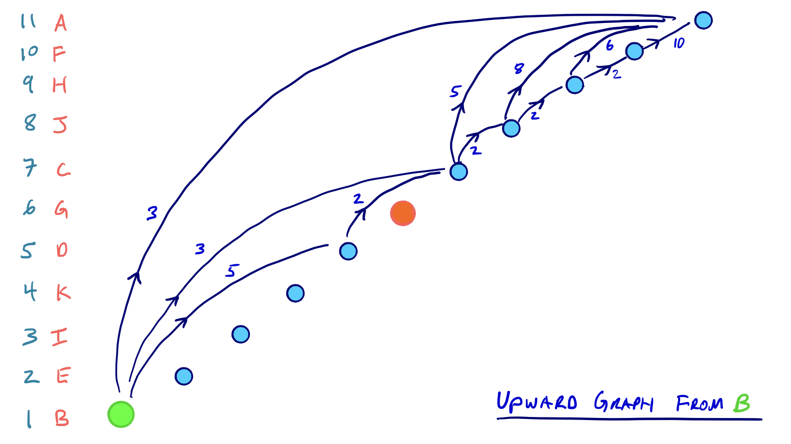
From our example above, let’s say our source node is \(B\) and our target node is \(G\). Then the two respective search spaces on \(G_{up}\) will look as follows:
Although we said that every edge in \(G*\) is either in the \(G_{up}\) or the \(G_{down}\) graph, not all edges […] will be relevant in the search space from a given node.
In our example above, for example, the edge \(E,D\) does exist in \(G_{up}\) since \(E\) was contracted before \(D\). But, because there is no path to \(E\) in either of the two searches from \(B\) or \(G\), we would never need to consider the edge \(E,D\).
Then on both of these upward graphs, we run a complete Dijkstra search, meaning that all nodes in both subgraphs must be settled. And it should be evident that in both searches, the number of settled nodes and relaxed edges is significantly reduced than if we were searching on the entire \(G*\) graph.
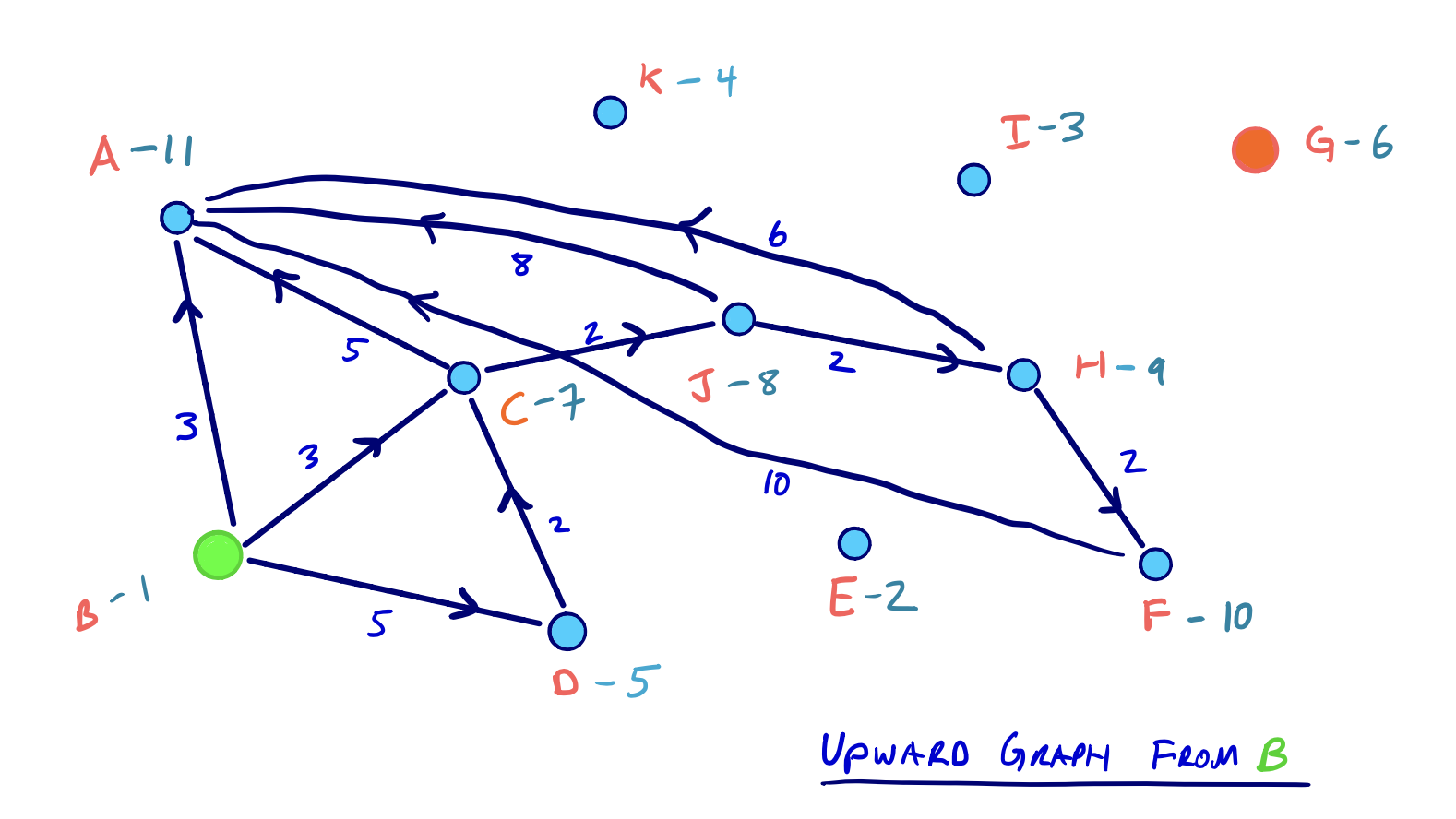
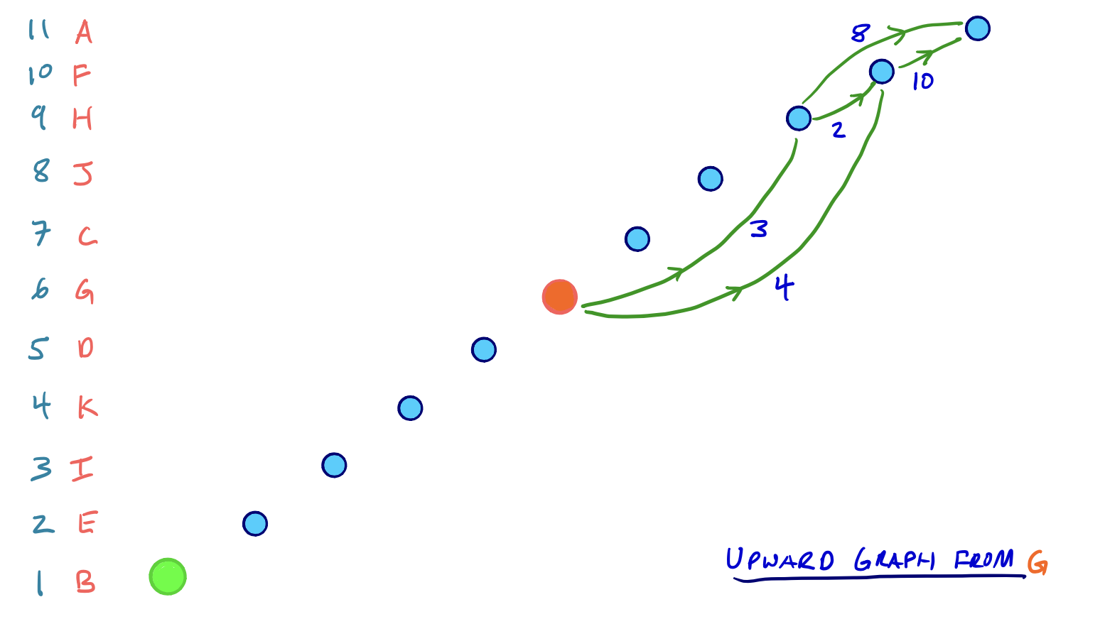
Moreover, because we have a complete ordering of nodes, the two search spaces can both be conceptualized as DAGs (directed acyclic graphs [Directed acyclic graph]) and are inherently topologically sorted [Topological order]. Consider the redrawing of the two searches that emphasizes this hierarchical nature of the contraction order:
[…]
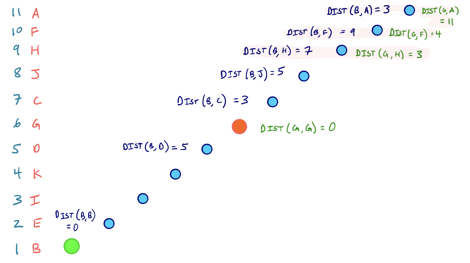
In any case, after running two complete Dijkstra searches on \(G_{up}\) from both the source and target, we have a set of nodes that are settled in both searches. We denote this set as \(L\).
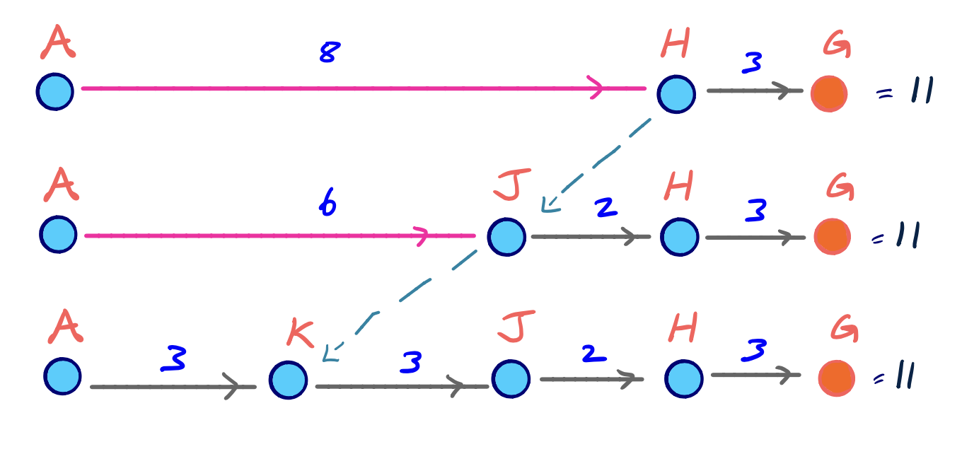
Continuing with our example from above, we see the nodes in \(L\) shaded in red with their corresponding shortest path scores:
This means the shortest path from \(B\) to \(G\) is 10 and goes through node \(H\).
[formatting mine]
Unpacking the shortest path from a shortcut
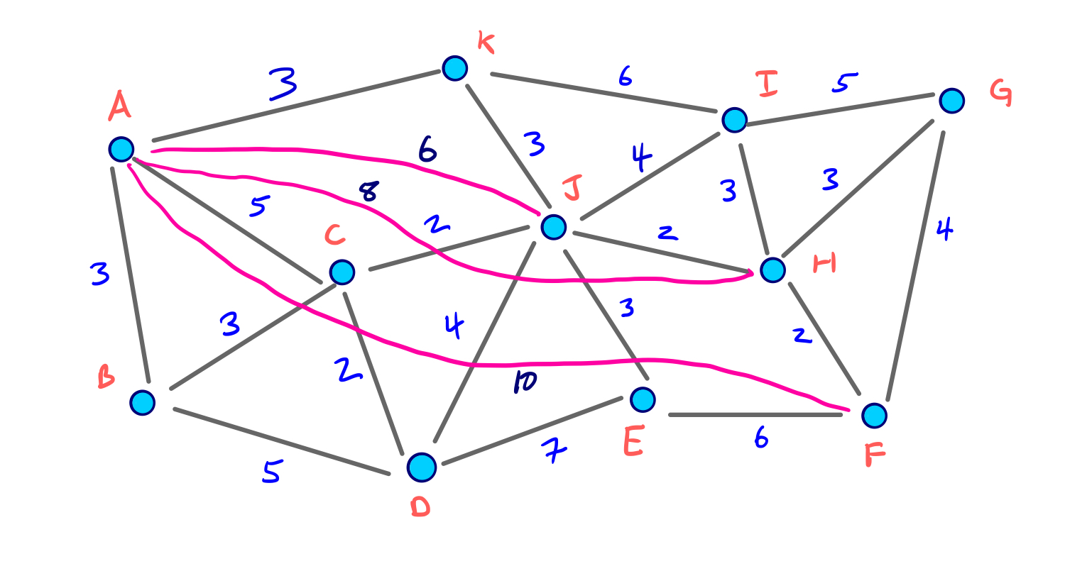
We’re able to compute the length of the shortest path, but we still need to unpack the actual arcs used on that path. We can handle this during the stage of contraction when shortcut edges are added. When we add a shortcut edge from \(u\) to \(w\) during the contraction of \(v\), we store a shortcut pointer to \(v\).
We then begin unpacking the shortest path on the G*U graph from the highest order node, in both directions. We back-trace parent edge pointers as in a regular Dijkstra algorithm, and if the parent edge has a shortcut pointer, we replace the parent edge with the shortcut edge, and continue to recursively unpack the full path.
Our example query above didn’t end up using any shortcut edges in \(G*\), but consider if we had queried the shortest path from node \(A\) to \(G\). Then, we would certainly use the shortcut edge \(A,H\). And since \(A\) is the highest-ordered node in terms of contraction time, we can visualize the ‘unpacking’ of shortcut edges as:
[Paraphrased, Spelling corrected]

Choosing a node order
Our query is correct no matter the order in which nodes were contracted, but a good node ordering has major implications for the performance of the queries. The order in which nodes are contracted affects the shortcut edges that do or don’t get added in G*. And as it’s been mentioned before, too many shortcut edges means too dense a G* graph and slower queries as a result.
Cost functions
Edge difference
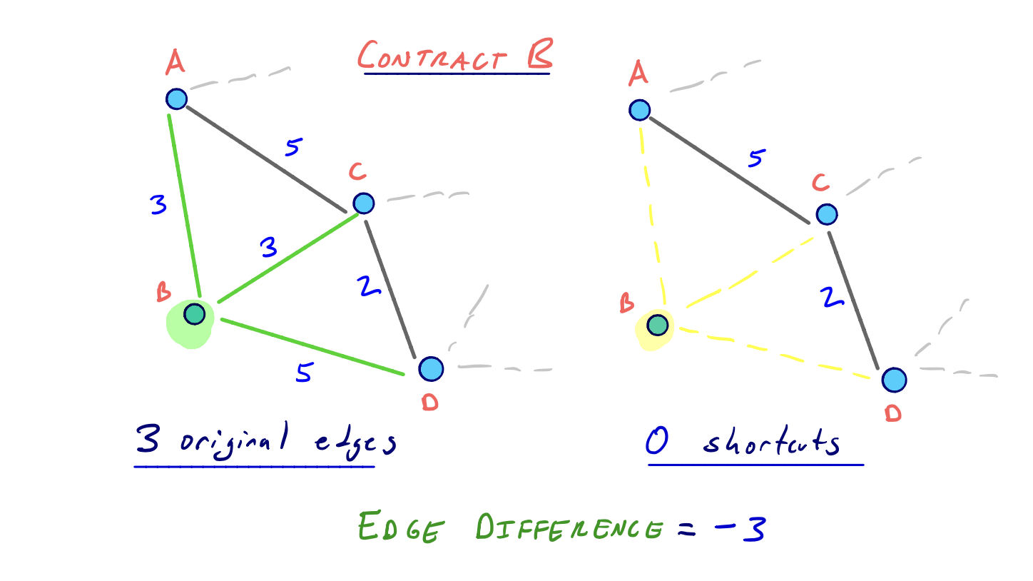
It turns out that the main function used to determine this cost involves simulating the contraction of each node. Given that all edges incident to a node are removed during contraction, we’re interested in the edge difference of a node, which is the difference between the number of original edges removed and the number of shortcut edges added.
[…]
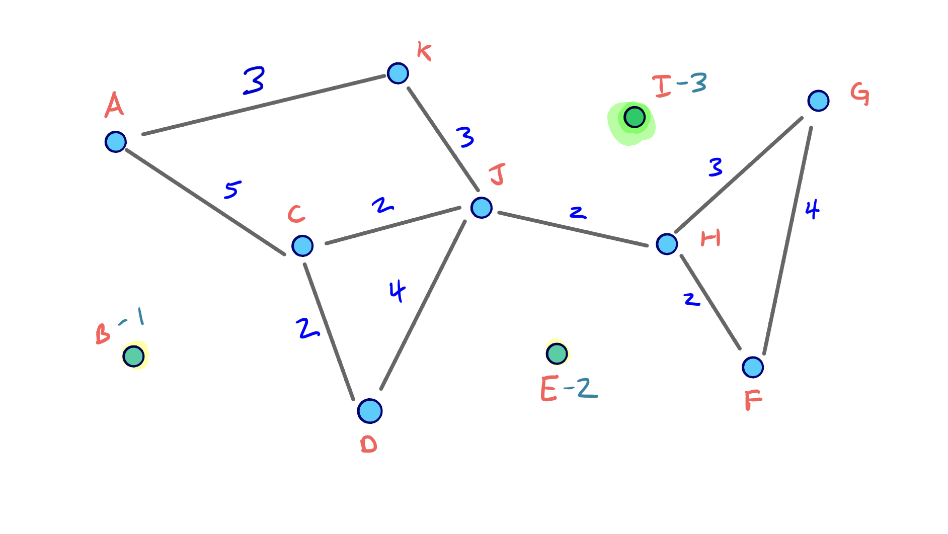
Using our original, arbitrary node ordering, we only added 3 shortcut edges. In the example, B was the first node we contracted, and it didn’t require any shortcuts to be added. In other words, the edge difference of B is -3.
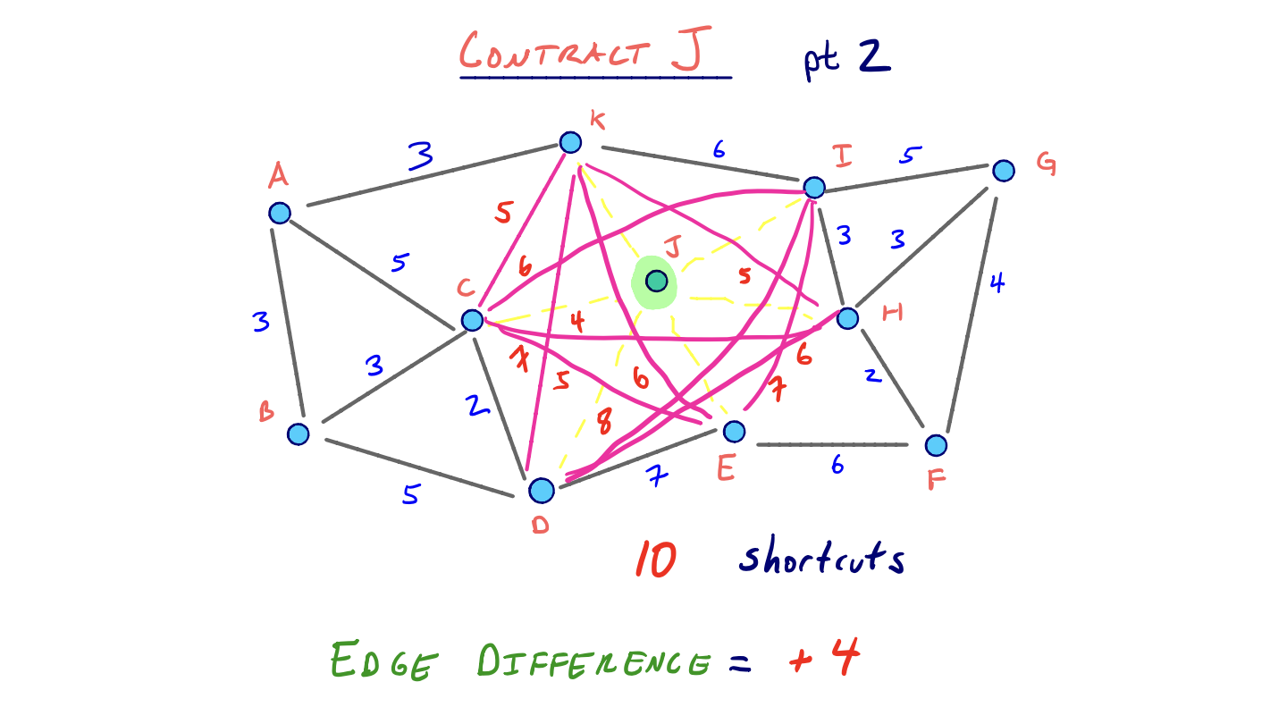
But what if we had first contracted J first? Compare what choosing J over B looks like:
So clearly J has a much greater edge difference than B, and so J is less attractive to contract early on.
[…]
But consider that after we begin contracting nodes, the edge difference for other nodes can be affected. If we wanted to strictly adhere to an ordering based on edge difference, we would need to recompute the edge difference for every remaining node in the graph after each contraction. Of course, this would end up taking quadratic time, so it isn’t feasible. Instead, we can use the lazy update heuristic […]
[…]
Before contracting the next minimum node, we recompute its edge difference. If it’s still the smallest in the priority queue [Priority queue], we can go ahead and actually contract it. If its edge difference is no longer the min, then we update its cost and rebalance our [priority queue]. We then check the next minimum node and continue this process.
Contracted neighbors
[…] we might consider the idea of uniformity to be important when contracting nodes. This means varying the location of nodes in terms of their contraction order.
Conceptually, we wouldn’t want to contract all nodes in a small region of the graph consecutively because we could risk adding too many wasteful shortcuts. In our original example, we had a pretty good ordering partly because nodes in different parts of the graph were contracted each round.
So an additional term to consider is the number of contracted neighbors each node has. This just involves counting the number of neighbors in the original graph that have already been contracted. When dealing with multiple terms like contracted neighbors and edge difference to determine cost, we would use a linear combination of terms.
Describe
| position | ease | box | interval | due |
|---|---|---|---|---|
| front | 2.50 | 5 | 36.62 | 2023-07-22T04:17:01Z |
| back | 2.65 | 4 | 15.61 | 2023-06-26T06:42:13Z |
Back
A speed up method for calculating the shortest path between nodes in a graph based on the assumption that some vertices are more important than others.
Source
(“Contraction Hierarchies” 2023)
Algorithm
| position | ease | box | interval | due |
|---|---|---|---|---|
| front | 2.20 | 4 | 12.26 | 2024-03-04T23:49:50Z |
| back | 2.5 | -1 | 0 | 2023-06-15T15:20:40Z |
Node contraction in Contraction hierarchies
Back
Given:
- \(v\): the vertex to contract
- \(U\): the set of all vertices with edges incoming to \(v\)
- \(W\): the set of all vertices with incoming edges from \(v\)
Steps:
- \(\forall\; u \in U\):
- \(\forall\; w \in W\):
- Compute \(P_{w} = \operatorname{weight}(u, v) + \operatorname{weight}(v, w)\)
- \(P_{max} = \operatorname{max}(P_w)\)
- \(\forall\; w \in W\):
- Perform a standard Dijkstra’s shortest-path [Single-pair shortest path problem] search from \(u\) to \(w\) on the subgraph excluding \(v\). Halt when we settle (1) a vertex with a shortest-path score \(> P_{max}\) or (2) \(w\).
- Add a shortcut if \(P_w < \operatorname{distance}(u, w)\)
- \(\forall\; w \in W\):
Source
Cloze
| position | ease | box | interval | due |
|---|---|---|---|---|
| 0 | 2.50 | 5 | 35.59 | 2024-03-12T06:45:40Z |
| 1 | 2.5 | -1 | 0 | 2023-06-15T15:21:11Z |
{{Node contraction}@0} is the process of {{finding shortcuts in a graph in Contraction hierarchies}@1}.
Source
(“Contraction Hierarchies” 2023)
Describe (Contraction hierarchies)
| position | ease | box | interval | due |
|---|---|---|---|---|
| front | 2.20 | 5 | 27.43 | 2024-03-18T08:19:33Z |
| back | 2.5 | -1 | 0 | 2023-06-15T15:30:07Z |
When do we contract a vertex, \(v\)?
Back
- Given a given vertex, \(v\)
- Let \(U\) be the set of vertices with edges going to \(v\)
- Let \(W\) be the set of vertices with edges coming from \(v\)
We contract \(v\) when the path \(u, v, w\) is the shortest path from \(u\) to \(w\).
Source
Describe (Contraction hierarchies)
| position | ease | box | interval | due |
|---|---|---|---|---|
| front | 2.50 | 6 | 87.92 | 2024-05-18T13:51:31Z |
| back | 2.5 | -1 | 0 | 2023-06-15T15:49:21Z |
How do we ensure \(u, v, w\) is the shortest path from \(u\) to \(w\)?
Back
Perform a local Dijkstra’s algorithm and compare the shortest path found excluding \(v\) to the shortest path found which includes \(v\).
Source
Describe (Contraction hierarchies)
| position | ease | box | interval | due |
|---|---|---|---|---|
| front | 2.35 | 7 | 203.08 | 2024-09-12T17:46:17Z |
| back | 2.5 | -1 | 0 | 2023-06-16T23:05:25Z |
How to extract the shortest path through an added shortcut?
Back
We store a pointer to the interim vertex, \(v\), when we contract \(u, v, w\) into \(u, w\).
Source
Describe (Contraction hierarchies)
| position | ease | box | interval | due |
|---|---|---|---|---|
| front | 1.90 | 3 | 6.00 | 2024-02-20T15:00:32Z |
| back | 2.50 | 1 | 1.00 | 2024-02-14T14:39:30Z |
Heuristics for choosing the order to contract vertices.
Back
Source
Describe (Contraction hierarchies)
| position | ease | box | interval | due |
|---|---|---|---|---|
| front | 2.20 | 5 | 25.66 | 2024-03-02T08:28:50Z |
| back | 2.5 | -1 | 0 | 2023-06-16T23:22:44Z |
Edge difference
Back
- Heuristic for deciding the order to contract vertices in a graph
- Ranks vertices by the number of edges removed by contraction
- \(\text{score} = \text{edges removed} + \text{edges (shortcuts) added}\)
Source
Describe (Contraction hierarchies)
| position | ease | box | interval | due |
|---|---|---|---|---|
| front | 2.20 | 6 | 67.93 | 2024-02-14T16:02:48Z |
| back | 2.50 | 1 | 1.00 | 2024-02-08T15:06:13Z |
Contracted neighbors
Back
- Heuristic for deciding the order to contract vertices in a graph
- Ranks vertices by the proximity of other contracted vertices
Source
Cloze (Contraction hierarchies)
| position | ease | box | interval | due |
|---|---|---|---|---|
| 0 | 2.35 | 3 | 6.00 | 2023-12-11T14:25:22Z |
We should contract vertices in {{ascending order}{direction}@0} of edge difference.
Source
Cloze (Contraction hierarchies)
| position | ease | box | interval | due |
|---|---|---|---|---|
| 0 | 2.50 | 5 | 33.68 | 2024-01-23T07:41:18Z |
We should contract vertices with {{fewer}{comparison}@0} contracted neighbors first.
Source
Describe (Contraction hierarchies)
| position | ease | box | interval | due |
|---|---|---|---|---|
| front | 2.20 | 7 | 130.70 | 2024-03-27T08:31:39Z |
| back | 2.50 | 2 | 2.00 | 2023-08-25T16:36:13Z |
Lazy update in the context of vertex ordering
Back
- Contracting any vertex may change the optimal contraction ordering of the remaining vertices
- Re-compute the rank/weight after popping the next vertex off the Priority queue
Source
Describe (Contraction hierarchies)
| position | ease | box | interval | due |
|---|---|---|---|---|
| front | 2.50 | 6 | 87.37 | 2024-05-21T00:41:19Z |
| back | 2.5 | -1 | 0 | 2023-06-20T15:35:52Z |
Query phase
Back
- Performs a bi-directional Dijkstra search for shortest path from \(s\) to \(t\)
- Forward search on upward graph from \(s\)
- Backward search on downward graph from \(t\)
Source
Cloze (Contraction hierarchies)
| position | ease | box | interval | due |
|---|---|---|---|---|
| 0 | 2.20 | 2 | 2.00 | 2023-11-01T14:52:43Z |
| 1 | 2.5 | -1 | 0 | 2023-06-20T15:38:35Z |
{{\(G_{up}\)}@0}, a subgraph of \(G\), contains only edges from \(v\) to \(w\) {{where we contracted \(w\) after \(v\)}{condition}@1}
Source
Cloze (Contraction hierarchies)
| position | ease | box | interval | due |
|---|---|---|---|---|
| 0 | 2.65 | 4 | 15.02 | 2023-12-13T15:19:55Z |
| 1 | 2.5 | -1 | 0 | 2023-06-20T15:39:08Z |
{{\(G_{down}\)}@0}, a subgraph of \(G\), contains only edges from \(v\) to \(w\) {{where we contracted \(v\) before \(w\)}{condition}@1}
Source
Describe (Contraction hierarchies)
| position | ease | box | interval | due |
|---|---|---|---|---|
| front | 2.20 | 7 | 144.13 | 2024-06-15T17:56:54Z |
| back | 2.5 | -1 | 0 | 2023-06-20T15:42:14Z |
How to unpack the shortest path from a shortcut
Back
Store a pointer to the contracted node, \(v\), whenever we contract \(u, v, w\) into \(u, w\).
Source
Witness path (Contraction hierarchies)
| position | ease | box | interval | due |
|---|---|---|---|---|
| front | 2.20 | 4 | 12.76 | 2024-03-04T10:08:23Z |
| back | 2.5 | -1 | 0 | 2023-06-20T15:44:41Z |
A path \(u, \dots, w\) around \(v\) with cost smaller than the cost of \(u, v, w\).
Source
(“Contraction Hierarchies” 2023)
Cloze (Contraction hierarchies)
| position | ease | box | interval | due |
|---|---|---|---|---|
| 0 | 2.50 | 6 | 96.97 | 2024-05-02T14:01:46Z |
Contraction is {{iterative}{process}@0}
Source
(“Contraction Hierarchies” 2023)